
Some prerequisites: some exposures with classical field theory would help
1. Introduction
For definiteness, let us study scalar field on flat 


As physicists, we should already be familiar with viewing
2. Klein-Gordon Lagrangian
To describe

let us define a map

such that 
such that
In general, a multiplication between two functions 


This is a typical definition of multiplication of scalar functions in the context of differential geometry. Let us also define some differentiations. The function

is defined as [I hope I do not need to make use of 

Sometimes, it is more convenient to write 


whose LHS is mentally irritating. Let us also define

such that

The functions 


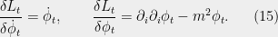
With the above ingredients, the Klein-Gordon Lagrangian is given by

It is a functional of 

On the other hand, direct computation gives

where we used the identity 
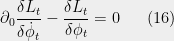
gives

which is Klein-Gordon equation.
Note the version of Euler-Lagrange’s equation (16). This version is often seen in Classical Mechanics but rarely appeared in Classical Field Theory. Physics students are often introduced to Classical Field Theory along the line of “Like in Classical Mechanics, there is also Euler-Lagrange’s equation. But we have to proceed differently to get Euler-Lagrange’s equation

which is tailored-made for Classical Field Theory”. From my direct experience, this approach makes Classical Field Theory to look far more complicated than Classical Mechanics and that there is an unforeseeable gap between them which cannot easily be filled in.
So hopefully our use of Euler-Lagrange’s equation (16) should make the connection between Classical Mechanics and Classical Field Theory a bit clearer.
3. Klein-Gordon Hamiltonian
To obtain Hamiltonian, we first look for conjugate momenta of 

Hamiltonian is then the functional of 

Let us next compute Poisson’s bracket. In the case of Classical Field Theory, we are often taught to start from the identity

where 
For this, let us view 


are vectors on 

where 
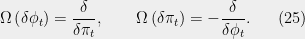
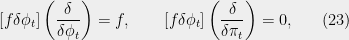
Let us define a vector field (called Hamiltonian vector field) of a scalar function 

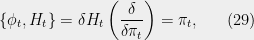
So it can be shown that Poisson’s bracket of scalar functions 

We want to compute 

So

4. Solution to equation of motion
This section is not so related to the title of the post. This means that we do not make use of any geometrical methods in the analysis [It might be possible to use one, but I still do not have enough knowledge to do so or to see if it is really possible]. However, I include this section just to make this post a bit more complete.
From either Lagrangian or Hamiltonian analyses, we obtain equation of motion for 

Recall that LHS of this equation is in fact a function 


Substituting this into the equation of motion (31) (whose LHS is already applied to 

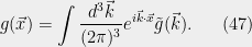
By inverse Fourier transforming, we obtain

For each 

But reality condition 


This gives

Sometimes, it is preferable to write RHS in terms of relativistic quantities. Based on the insight from Special Relativity, one could expect to put 


The exponent is already in the relativistic form: 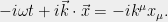
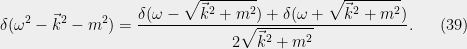
So by using the fact that 


The coefficient would look nicer if we set
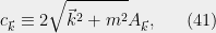
[NB: This choice has no physical motivation. It just only makes the presentation a bit nicer. The choice which often appears in Classical Field Theory is 

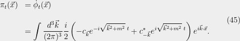
Perhaps this form is the most relativistic that one could get. As a cross-check, one could integrate out

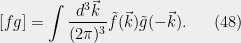
Let us substitute the solution into the Hamiltonian (20). For this, it is convenient if we first rewrite

Then we compute
Any well-behaved functions

Direct computation gives
Using this identity, it is easy to show that


Combining these results give
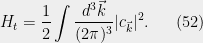
So Hamiltonian of the system is time-independent.
Let us simply end this post here.
